Topic Modeling with MALLET¤
Overview¤
Topic modeling is a statistical method for discovering abstract themes or "topics" within a collection of documents. MALLET is a mature tool for topic modeling used widely in the Humanities. It is a Java package that needs to be installed separately from Lexos. The Lexos mallet module provides a straightforward wrapper for running MALLET, managing outputs, and creating visualizations of your topic model.
The Lexos mallet module integrates Maria Antoniak's Litte Mallet Wrapper functions with a slightly simplified API that manages file paths. For more advanced methods of exploring a topic model, see the Lexos integration of DFR Browser 2.
In the examples below, we will use a sample dataset of English-language fiction from David Bamman's LitBank. Additional texts were collected by Allen Riddell for TAToM: Text Analysis with Topic Models for the Humanities and Social Sciences.
Installing MALLET¤
MALLET does not come packaged with Lexos; it must be installed separately. Lexos can interface with MALLET through one of two backends: a wrapper for the original Java-based MALLET binary or through David Mimno's more recent port of MALLET to Rust, which is accessible through the PyRMallet Python binding. The latter has a much simpler installation procedure.
Using the Java Backend¤
To use the original Java-based MALLET binary, you need to download and install MALLET from its official website. Once installed, ensure that the MALLET binary is accessible from your system's PATH or note its installation path for later use. You will also need to have the Java Developer's Kit (JDK) installed on your system. For useful account of the installation procedure, Shawn Graham, Scott Weingart, and Ian Milligan's tutorial Getting Started with Topic Modeling and MALLET.
After installation, you should verify that MALLET is correctly installed and accessible from your system's PATH. For instance, if your MALLET binary is located at ~/mallet/bin, you can run the following command in a terminal:
If you are using a Jupyter notebook, you can configure the path to your MALLET binary and run
If you receive a list of commands, MALLET is installed and the path is correct. Alternatively, on the command line, you can type the path to your MALLET binary and hit Enter. You should see the same list of commands.
Using the PyRMallet Backend¤
PyRMallet is a Python binding for David Mimno's Rust port of MALLET, which simplifies the installation process compared to the original Java-based MALLET binary. To use PyRMallet, you need to do is install it via pip:
or, if you are using uv, you can add it to your environment with
Import the Mallet class from the mallet Module¤
First, import the Mallet class and helper functions from the Lexos mallet module.
Load Your Data¤
Your data must take the form of a list of strings or spaCy Doc objects. Example data:
sample_docs = [
    "The quick brown fox jumps over the lazy dog.",
    "Never jump over the lazy dog quickly.",
    "A fast brown fox leaps over sleeping dogs.",
    "Dogs are great pets for families.",
    "Foxes are wild animals found in forests."
]

training_data = import_docs(sample_docs)
This just copies the list sample_docs into a new list called training_data but ensures that the raw text strings are copied if your sample docs are spaCy Doc objects.
Because topic modelling normally uses a large number of documents, you will most likely want to import them from a directory or line-delimited file. The read_dirs() and read_file() functions will read your documents into a list of strings.
Reading Directories¤
The read_dirs() function will read all text files in a directory (or list of directories) into a list of strings where each file is treated as a separate document. Note that the order of the documents in the list is important, as it will be used for document indexes in the topic model.
In the examples below, we will use the litbank_texts folder distributed with MALLET, which contains text from 12 Wikipedia articles.
from lexos.topic_modeling.mallet import read_dirs
corpus_dir = "litbank_texts"
training_data = read_dirs(corpus_dir)
Reading from a File¤
You can also load documents from a single file using the read_file() function. Here each line in the file is treated as a separate document. Again, the order of documents will be used for document indexes in the topic model.
Note: Technically, MALLET expects the tab-delimited file where the first column is an index, the second is an optional label, and the third is the document text itself. The read_file() function accepts files in this format, as well as files containing only texts.
from lexos.topic_modeling.mallet import read_file
corpus_file = "sample_data.txt"
training_data = read_file(corpus_file)
Train a Topic Model¤
You are now ready to train a topic model. This involves three steps:
- Create a topic model involves three steps illustrated below. First, create a
Malletinstance, providing it with the path to a directory to save the model and, if required (see above), the path to your Mallet binary file. - Next, import your data with the
import_data()method. - Finally, train the topic model.
The model metadata property returns a dictionary containing paths to output files and model statistics.
Start by creating a Mallet instance:
model_dir = "mallet_model"
path_to_mallet = "/path/to/your/mallet/binary"
mallet_model = Mallet(model_dir=model_dir, path_to_mallet=path_to_mallet)
Note
By default, the Mallet class uses the Java backend and requires path to your MALLET binary file. If you are using the PyRMallet backend, you do not need to provide the path to the MALLET binary (although a default path will be stored in your model's metadata).
Now import your training data into the model instance with import_data.
You can configure the following parameters:
keep_sequence: Keep the token sequence. Default isTrue.preserve_case: Preserve case. Default isTrue.remove_stopwords: Remove stopwords. Default isTrue.training_ids: A list of integers indicating the IDs of the documents you want to import. IfNone, all documents in your training data will be imported.
When you train a model, MALLET creates a "pipe" file that records the sequence of data processing steps (such as tokenization, stopword removal, case normalization, etc.). This file is saved in your model directory with the extension .mallet.
If you later want to import new documents for inference or further modeling, you can use use_pipe_from with the path to the .mallet file. This guarantees consistency between training and inference, so your new documents are handled identically to your training set.
Finally, train your model:
If verbose is set to True, you will see something like:
✔ Training topics...
Mallet LDA: 20 topics, 5 topic bits, 11111 topic mask
Data loaded.
max tokens: 147
total tokens: 1245
<10> LL/token: -9.11285
<20> LL/token: -8.87062
<30> LL/token: -8.71832
<40> LL/token: -8.61369

0       0.25    average Test energy Hill energies ended innings batsman day predictions accurate holds neutron
properties predict Dulong–Petit classical mechanics statistical handicapper
1       0.25    back Gilbert year actors drama Greek productions England movie accomplishments romance Actress
graduating retiring apex habitat introduction continent mainland commonly

...

Total time: 0 seconds

✔ Complete
This is a display of the state of your model after each iteration. It can be quite long, so it may be truncated in a notebook environment. If you are not interested in observing this output, you can set verbose=False.
The train() method takes the following parameters:
num_topics: The number of topics to train. The default is 20.num_iterations: The number of iterations to train for. The default is 100.optimize_interval: The interval at which to optimize the model. The default is 10.verbose: Whether to print the MALLET output showing the state at different iterations. The default isTrue.path_to_inferencer: Optional output filename for saving a trained inferencer object (see below). If not provided, defaults tomodel_dir/inferencer.mallet.
Loading an Existing Model¤
Sometimes you need to load an existing model into memory, rather than creating one from scratch. You can do this easily by instantiating a new Mallet object with the existing model_dir path.
# Import the Mallet class
from lexos import Mallet

# Initialize Mallet model
mallet_model = Mallet(model_dir="mallet_model")

# View the previously-generated metadata for the trained model
mallet_model.metadata

---

## After Training

After training, you can inspect various model properties:

- `mallet_model.metadata`: Returns a dictionary of information about the model, especially the paths and commands that were used to generate the model.
- `mallet_model.topic_keys`: A list of lists where each sublist is the topic keys for a given topic.
- `mallet_model.distributions`: A list of lists where each inner list is the topic distribution for a single document: how much each topic contributes to the document (sums to 1).
- `mallet_model.num_docs`: The number of documents used to generate the model.
- `mallet_model.vocab_size`: The number of unique terms used by the trained model.
- `mallet_model.mean_num_tokens`: The mean number of tokens per document.

These properties allow you to inspect the model, analyze results, and use outputs for further processing.

!!! note "Setting Metadata Values"
    In most cases, you will not want to change the metadata values, which are set automatically by class methods. However, in some cases you may wish to add additional information to the model's metadata, such as author or version number. Use the `set_metadata` method to do this.

    ```python
    mallet_model.set_metadata("author", "John Smith")
    mallet_model.set_metadata("version", "1.0")
    ```

    Any values you add with the `set_metadata` method will automatically be saved in the model's `meta.json` file and will be available if you need to reload the model (see below).

---

## Display Topics and Top Words

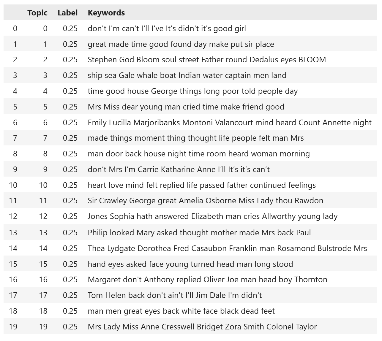
Once you have created your model, you can display the discovered topics and their top words using `get_keys()`. This method takes the following parameters:

- `num_topics`: The number of topics to get keys for. If `None`, get keys for all topics.
- `topics`: A list of topic indices to get keys for. If `None`, get keys for all topics.
- `num_keys`: The number of key terms to output for each topic.
- `as_df`: Whether to return the result as a pandas DataFrame instead of a string. The default is `True`.

```python
mallet_model.get_keys(as_df=True)
Custom Topic Labels
You can provide custom labels for your topics by adding a topic_labels dictionary to the model's metadata. This is useful for replacing the default labels with more topic descriptive titles, especially after using an LLM to generate them. An example of how to use AI-generated labels can be found at the end of this page.
The dictionary should map topic indices (as strings) to your custom labels. To add them to the model's metadata, use the set_metadata method, as shown below:
```python custom_labels = { "0": "Military & Strategy", "1": "Classical Literature", "2": "Scientific Discovery" }
Add the labels to the model's metadata¤
mallet_model.metadata["topic_labels"] = custom_labels mallet_model.set_metadata("topic_labels", custom_labels)
These labels will be now displayed in the results of get_keys and will be used in all the visualization methods produced by the Mallet class.
Display the Top Documents in Each Topic¤
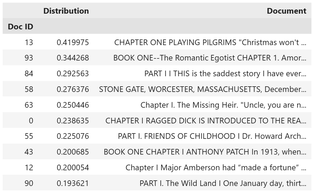
You can display the discovered topics and their top words using get_top_docs(). This method takes the following parameters:
topic: The topic number to display.n: The number of top documents to return.metadata: A Dataframe with the metadata in the same order as the training data. This can include information such as document labels.as_str: Whether to return the result as a string instead of a pandas DataFrame. The default isFalse.
Display the Topic Term Probabilities¤
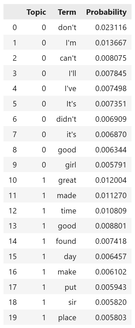
You can display the the term distribution for a given topic with get_topic_term_probabilities(). This method takes the following parameters:
topics: The topic number (or list of topic numbers) to display. If None, get the probabilities for all topics.n: The number of key terms to display.as_df: Whether to return the result as a string instead of a pandas DataFrame. The default isFalse.
Visualizing Topic-Term Weights with a Termite Plot¤
Visualizing Topic-Term Weights with a Termite Plot¤
The plot_termite() method creates a termite plot using MALLET topic-term weights and the textacy visualization API. This view is especially useful for comparing important terms across multiple topics at once. For more information on termite plots, see Chuang, Jason, Christopher D. Manning, and Jeffrey Heer. “Termite: Visualization techniques for assessing textual topic models.” Proceedings of the International Working Conference on Advanced Visual Interfaces. ACM, 2012.
The method takes the following parameters:
topics: Topic index or list of indices to include. IfNone, all topics are used.highlight_topics: Topic index, label, or list of topic indices/labels to visually emphasize.n_terms: Number of top terms to include in the plot.rank_terms_by: How terms are ranked before selection (for example,"max","mean","var").sort_terms_by: How selected terms are ordered in the display (for example,"seriation","weight","index","alphabetical").title: An optional title for the plot.output_path: Optional path for saving the figure.rc_params: Optional matplotlib style overrides passed totextacy.
ax = mallet_model.plot_termite(
    topics=[0, 1, 2, 3],
    highlight_topics=[1],
    n_terms=20,
    sort_terms_by="seriation",
    output_path="termite_plot.png"
)
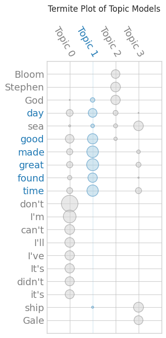
If output_path is omitted, the method returns the matplotlib axis so you can customize or display the figure in your notebook environment.
You can also use the plot_termite_plotly method to generate an interactive version. The Plotly version allows you to adjust the scaling of the circles with marker_scale. You can use this to minimize differences in appearance between the Plotly and the non-Plotly outputs.
fig = mallet_model.plot_termite_plotly(
    topics=[0, 1, 2, 3],
    highlight_topics=[1],
    n_terms=20,
    rank_terms_by="max",
    sort_terms_by="seriation",
    marker_scale=25, # The default setting is 25, which can make the circles appear too large in some cases. Adjust as needed.
)
fig.show()
The output_path parameter saves to an HTML file.
Visualizing Topic Probabilities by Category with Boxplots¤
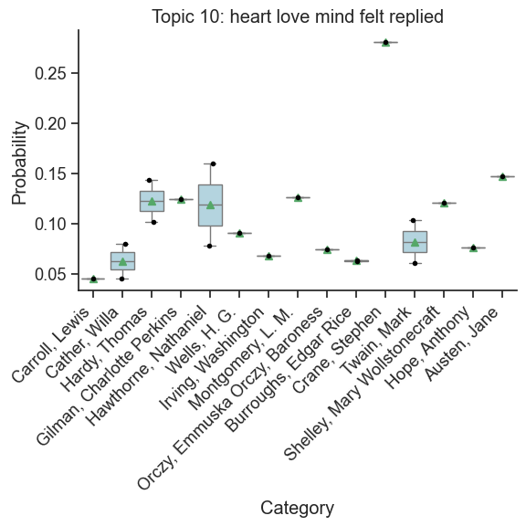
The plot_categories_by_topic_boxplots() method lets you visualize how topic probabilities are distributed across different categories (e.g., genres, labels, or other groupings). This is useful for understanding which topics are most associated with which categories in your data.
The function takes a number of parameters that allow you to choose your topics and categories, as well as to customize the appearance of the box plots.
categories: List of category labels for each document (must match the order of your training data).topics: Topic index or list of indices to plot. IfNone, all topics are plotted.output_path: Path to save the figure. IfNone, the plot is shown but not saved.target_labels: List of unique category labels to include. IfNone, all categories are included.num_keys: Number of top keywords to display in the plot title.figsize: Size of the figure (tuple, e.g.,(8, 6)).font_scale: Font scaling for the plot.color: Color for the boxplots (matplotlib color name or object).show: Whether to display the plot (True) or just return the figure object (False).title: Custom title for the plot. If not provided, a default is used.overlay: How to display individual data points ('strip','swarm', or'none').overlay_kws: Dictionary of keyword arguments for the overlay plot (e.g., point size, color).
Overlay advice:
- Use
'strip'(default) for most cases, especially when you have a moderate number of documents per category. It shows individual points with jitter for visibility. - Use
'swarm'when you have a small number of documents and want to avoid overlapping points; it arranges points to minimize overlap. - Use
'none'if you only want to see the boxplot summary and not individual data points (useful for large datasets).
The cell below will run a basic example.
categories = ["People", "Concepts", "People", "People", "People", "Battles", "Texts", "Texts", "Animals", "Planets", "People", "People"]
mallet_model.plot_categories_by_topic_boxplots(categories)
Visualizing Topic-Category Associations with a Heatmap¤
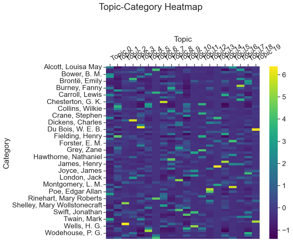
The plot_categories_by_topics_heatmap() method creates a heatmap showing how topics are distributed across different categories. This is useful for quickly spotting which topics are most associated with which categories, especially when you have many topics or categories. It takes the following parameters:
categories: List of category labels for each document (must match the order of your training data).output_path: Path to save the figure. IfNone, the plot is shown but not saved.target_labels: List of unique category labels to include. IfNone, all categories are included.num_keys: Number of top keywords to display in the topic labels.figsize: Size of the figure (tuple, e.g.,(10, 8)).font_scale: Font scaling for the plot.cmap: Colormap for the heatmap (e.g.,"rocket_r","viridis", or any matplotlib colormap).show: Whether to display the plot (True) or just return the figure object (False).title: Custom title for the plot. If not provided, a default is used.
categories = ["People", "Concepts", "People", "People", "People", "Battles", "Texts", "Texts", "Animals", "Planets", "People", "People"]
mallet_model.plot_categories_by_topics_heatmap(
    categories=categories,
    num_keys=3,
    figsize=(8, 6),
    font_scale=1,
    cmap="viridis",
    show=True,
    title="Topic-Category Heatmap"
)
Note
If you make the figure size too small, some topic labels may be omitted. You can mitigate this by reducing the font scale.
Visualizing Topics with Word Clouds¤
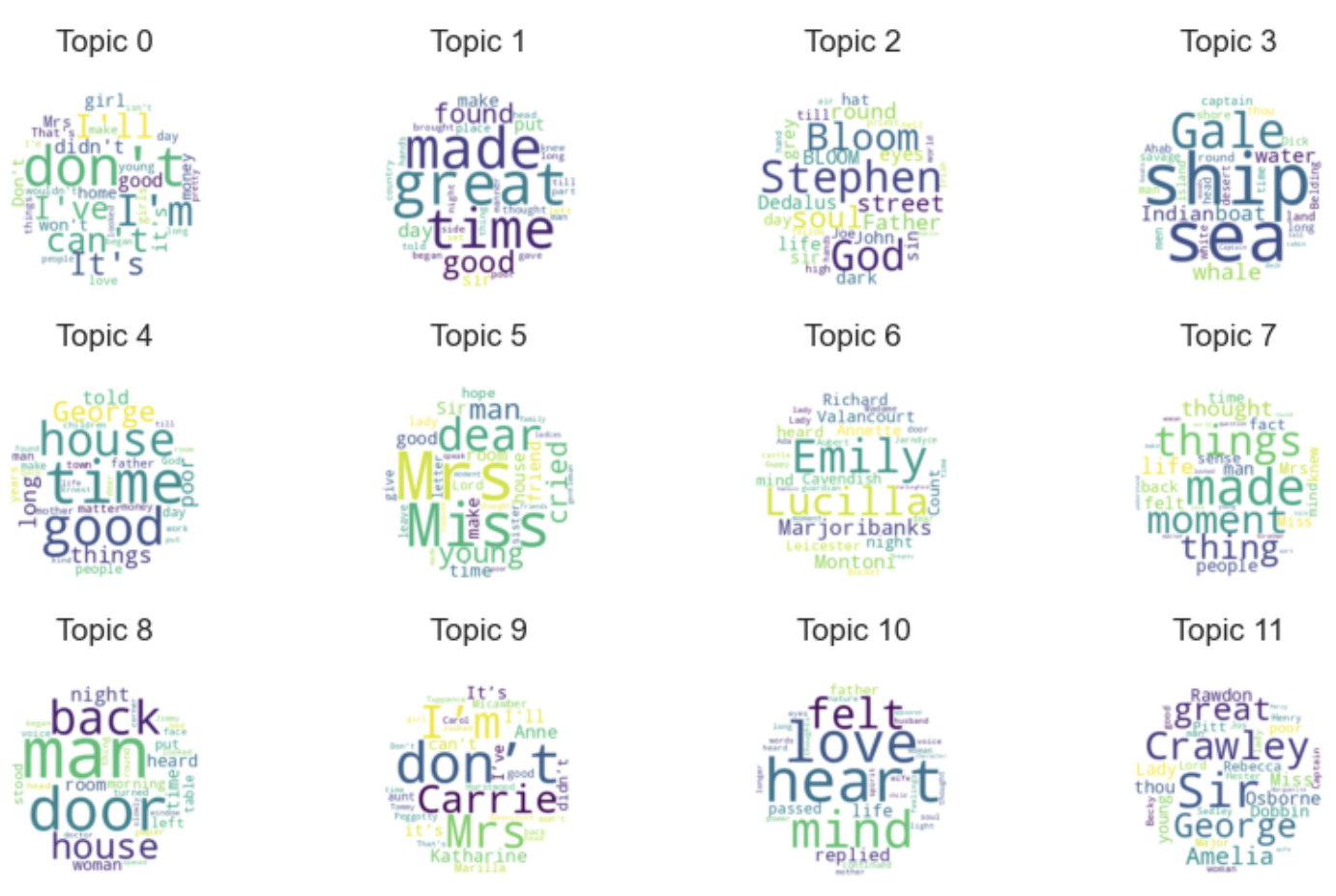
The topic_clouds() method in the Mallet class generates word clouds for each topic, providing a visual summary of the most important terms per topic. This is useful for quickly understanding the main themes captured by your model.
Parameters:
topics: A topic number or list of topic numbers to include. If None, all topics are shown.max_terms: An optional maximum number of keywords per topic cloud (default: 30).figsize: An optional tuple (default: (10, 10)) specifying the size of the overall figure.output_path: An optional string specifying the path to save the figure.show: An optional boolean. If True, displays the figure; if False, returns the matplotlib Figure object.round_mask: An optional boolean or integer indicating whether to use a circular mask for the clouds (True/False or integer radius).title: An optional string specifying the title for the figure.**kwargs: Additional keyword arguments for customization (see below).
Customization:
- Pass
optsin**kwargsto control word cloud appearance (e.g., background color, colormap). Accepts arguments for the Python wordcloud package. - Pass
figure_optsin**kwargsto control figure-level options usingmatplotlib(e.g., facecolor).
Visualizing Topic Trends Over Time¤
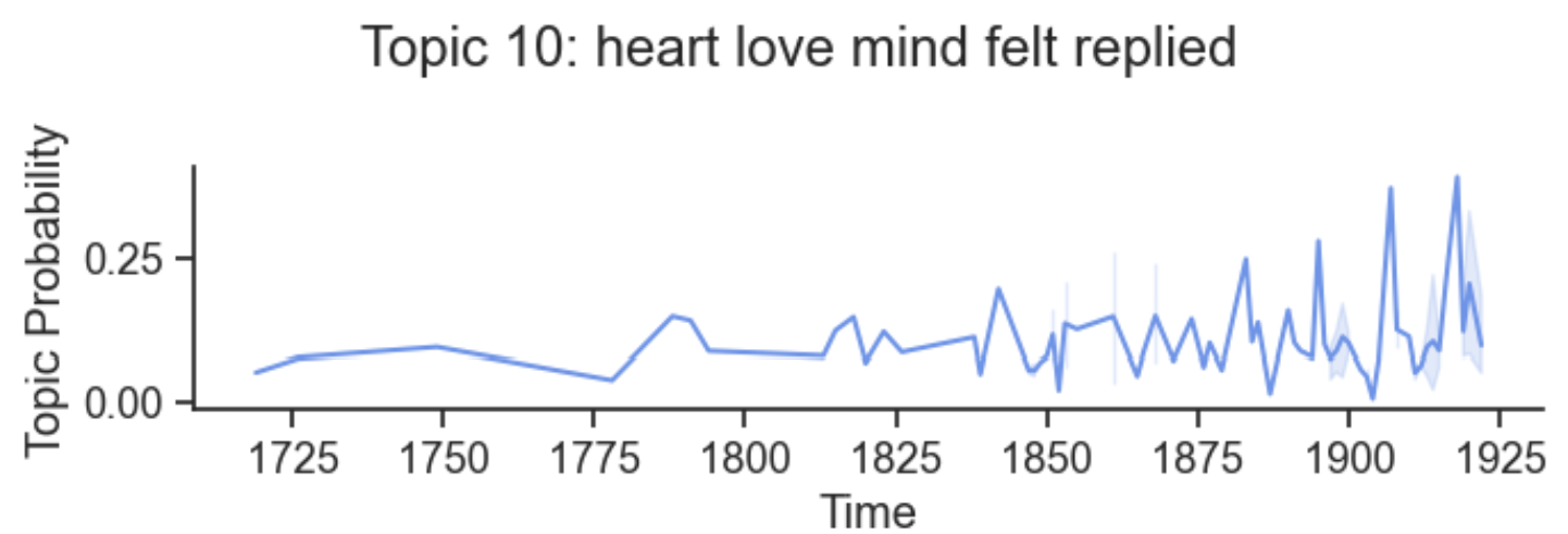
The plot_topics_over_time() method in the Mallet class allows you to visualize how the probability of a specific topic changes across a sequence of documents, such as those ordered by time or another variable. This is useful for exploring temporal or sequential patterns in your corpus.
Parameters:
times: A sequence of time points or other ordering variable, one per document.topic_index: An integer specifying the topic to plot (0-based index).topic_distributions: An optional list of lists of floats representing topic distributions per document. If None, uses the model's distributions.topic_keys: An optional list of lists of strings representing topic keys. If None, uses the model's keys.output_path: An optional string specifying the path to save the figure.figsize: An optional tuple specifying the size of the figure (default: (7, 2.5)).font_scale: An optional float specifying the Seaborn font scale (default: 1.2).color: An optional string specifying the line color (default: "cornflowerblue").show: An optional boolean. If True, displays the figure; if False, returns the matplotlib Figure object.title: An optional string specifying the title for the figure. If not supplied, uses topic keywords.
Note:
- The
timeslist must be the same length and order as the documents in the training data.
times = [2001, 2002, 2003, 2004, 2005, 2006, 2007, 2008, 2009, 2010, 2011, 2012]
mallet_model.plot_topics_over_time(times=times, topic_index=0, show=True)
Advanced Features¤
Infer Topics for New Documents¤
Sometimes you want train a model and then feed it new documents after training. To help you do this, Lexos creates an inferencer file when you initially train the model. It will automatically be saved as inferencer.mallet in your model's folder, but you can use the path_to_inferencer parameter when training your model (or change it in your metadata) if you want to give it a different name or save it somewhere else.
To use the inferencer to infer new topic distributions, you will need to define the following paths:
pipe_file: Path to the.malletpipe file created during training. Ensures new documents are processed identically to training data.output_path: Where to save the topic distributions for the new documents (as a text file).- path_to_inferencer`: Path to the inferencer file created during training. This is used to infer topics for new documents.
In the example below, we read three texts from the additional_texts folder and define our paths relative to out model directory.
# Read the new documents for inference
additional_dir = "additional_texts"
additional_docs = read_dirs(additional_dir)

# Define paths to your pipe file, output path, and inferencer file
pipe_file = mallet_model.model_dir / "training_data.mallet"
path_to_inferencer = mallet_model.metadata['path_to_inferencer']
output_path = mallet_model.model_dir / "new_doc_topics.txt"

# Use the Mallet class's infer() method to get topic distributions
inferred_topics = mallet_model.infer(additional_docs, path_to_inferencer=path_to_inferencer, use_pipe_from=pipe_file, output_path=output_path)

# Display the inferred topic distributions (also saved to the output_path)
print("First Two Distributions:")
for i, dist in enumerate(inferred_topics[:2]):
    print(f"Document {i}: {dist}\n")
This will output
Rewriting extended pipe from mallet_model/training_data.mallet
  Instance ID = aa26dc31-29d3-42b1-b4a1-89a31b9cb449
First Two Distributions:
Document 0: [0.03701587759523014, 0.22562284679833042, 0.011659133624194816, 0.002089723344164718, 0.05482355134447515, 0.3132625834708346, 0.0011246840846130227, 0.00875726731924916, 0.005425182463279581, 0.0013473854522018753, 0.1560084238479422, 0.014117284325535412, 0.10390895731894548, 0.005292742634827119, 0.0019167923579688285, 0.04280442602096767, 0.0013246091759711973, 0.004029924652703965, 0.008940321094880905, 0.0005282830736837843]

Document 1: [0.04276331790842658, 0.11287681572179306, 0.022736045794555307, 0.01648919393485762, 0.05502635415146537, 0.11588804624647527, 0.00856333391392494, 0.0890756981614076, 0.02915079847037649, 0.0010344730189665156, 0.18701993312212353, 0.012668273493168633, 0.012715348488343447, 0.041008989754911886, 0.011172857813115408, 0.15024808522457125, 0.006581476617065313, 0.00015573977570333965, 0.08273940381087777, 0.0020858145778706724]
Now combine the old and the new distributions. Since some of our visualization methods involve categories and times, we create categories and times lists that include our new documents.
# Combine training and new distributions
all_distributions = mallet_model.distributions + inferred_topics

# Create a combined categories list (must match the length and order of all_distributions)
new_categories = ["Brontë, Charlotte", "Brontë, Charlotte", "Richardson, Samuel"]
all_categories = categories + new_categories

# Create a combined times list (must match the length and order of all_distributions)
new_times = [1846, 1853, 1740]
all_times = times + new_times
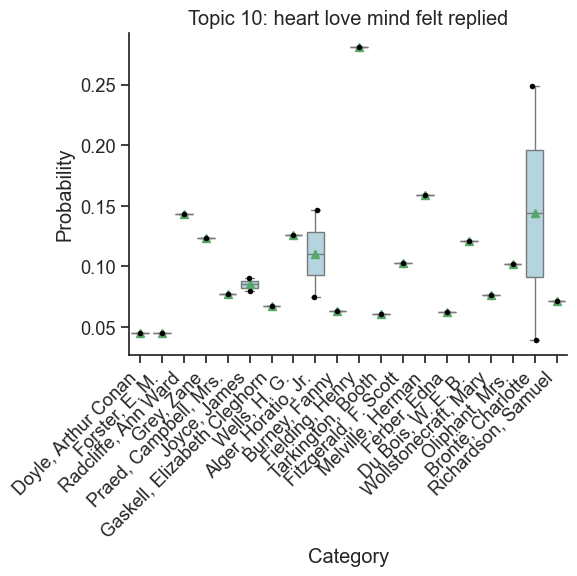
Now we can use any of the visualization methods. For instance, here are boxplots for the combined distributions:
mallet_model.plot_categories_by_topic_boxplots(
    topics=3,
    categories=all_categories,
    topic_distributions=all_distributions,  # Pass the combined distributions
    show=True
)
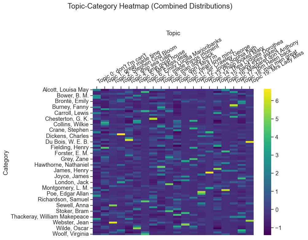
The code below will produce heatmap and topic over time visualizations.
mallet_model.plot_categories_by_topics_heatmap(
    all_categories,
    topic_distributions=all_distributions,
    num_keys=3,
    figsize=(8, 6),
    font_scale=1,
    cmap="viridis",
    show=True,
    title="Topic-Category Heatmap (Combined Distributions)"
)
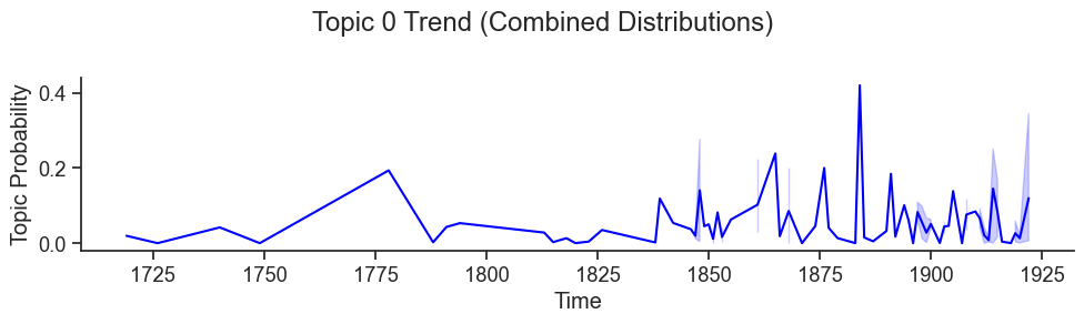
times = [1846, 1853, 1740]
mallet_model.plot_topics_over_time(
    times=all_times,
    topic_index=0,
    topic_distributions=all_distributions,
    title="Topic 0 Trend (Combined Distributions)",
    color="blue",
    figsize=(10, 3),
    show=True
)
Automatic Topic Labelling with LLMs (Experimental)¤
Lexos supports automatic topic labelling using LLM providers like OpenAI, Google Gemini, and Anthropic Claude, as well as local models via OpenAI-compatible APIs (like Ollama).The LLM labelling feature is experimental and may not work with all models or configurations.
Warning
Generative AI models can produce idiosyncratic, duplicate, misleading, or incorrect results. It is highly recommended that you inspect the topic labels and modify any generated labels manually, as appropriate.
First, configure the TopicLabelerConfig. You must provide either an api_key (for cloud providers) or a base_url (for local providers). Attempting to create a configuration without one of these will raise a validation error.
By default, the prompt sent to the LLM is as follows:
Analyze the following high-frequency words from a topic model cluster:
Words: [the list of words in the topic]
Contextual context snippet: [an optional text snippet supplied with the `documents_snippet` parameter]
Provide 1 concise, clear title/label (3-5 words max) summarizing this topic.
Return ONLY the plain text label without any preamble or quotes.
You can send a custom prompt to the LLM by providing a string to the prompt parameter. The list of words in each topic will be appended to your prompt. You can also provide an optional snippet of text from your documents with the documents_snippet parameter, which will be included in the prompt to provide context for the LLM. This is especially useful if your topics are highly abstract or if you want to provide additional context for the LLM to consider when generating labels.
You can further modify the labelling process with the following parameters:
max_tokens: The maximum number of tokens to return in the response. The default is 50 to keep labels short.temperature: The temperature for the LLM. The default is 0.1, specifies low creativity. You can increase it to 1 until you find a balance between creativity and consistency in the labels.timeout: The timeout for the LLM request in seconds. The default is 120 seconds, which may be too short for some models or prompts (especially if running in a Jupyter notebook). You can increase this if you are experiencing timeouts.max_retries: The maximum number of retries for a failed LLM request (such as due to rate limits for cloud-based services).include_reasoning: Whether to include the model's reasoning in the response in "thinking" mode. The default isFalse, which is recommended for most models to reduce the number of tokens used and speed up the labelling process. If you are able to accommodate larger numbers of tokens without timeouts, you can set this toTruefor better results.
Depending upon which LLM you choose, you may have to play around with the settings a lot to obtain clean and consistent feedback -- especially when using a local model -- in a reasonable amount of time.
Here is an example of how to use the LLM labeler with a local model.
from lexos.topic_modeling.mallet.llm_labeler import TopicLabelerConfig, label_mallet_topics

sample_prompt = (
    f"Analyze the high-frequency words from an LDA topic model cluster in the list below:\n"
    f"Provide 1 concise, clear label (3-5 words max) summarizing this topic. "
    f"Return ONLY the plain text label without any preamble or quotes."
)

# Configure the labeler for a local model
config = TopicLabelerConfig(
    provider="local", # Should be local for local models
    model="llama-3.2-1b-instruct",
    base_url = "http://172.17.160.1:1234/v1/chat/completions", # Required for local models
    max_tokens = 512,
    temperature = 0.25,
    prompt=sample_prompt
)

# Specify the path to the topic keys file generated by your trained Mallet model
topic_keys_path = mallet_model.metadata["path_to_topic_keys"]

# Specify topic numbers to label or None for all topics
topic_nums = None # Or use a zero-indexed list like [0, 1]

# Generate the topic labels mapping from your trained Mallet model using the LLM labeler
topic_labels = label_mallet_topics(topic_keys_path=topic_keys_path, config=config, topic_nums=topic_nums)
The output is a dictionary mapping topic indices to the generated labels. You can inspect the labels and modify them as needed.
With a cloud-based model, use a configuration like the one below:
config = TopicLabelerConfig(
    provider="gemini",
    model="gemini-3.6-flash",
    api_key="your_api_key", # Required for cloud providers
    max_tokens = 512,
    temperature = 0.1,
)
Change any labels you want Once you are satisfied with the labels, you can commit them to your topic model instance by adding them to the metadata "topic_labels" key.